Making the right choice is a difficult task in many fields of life and business. It gets even harder as the number of variables increases. In the data science field, this increase in problem complexity is called the ‘curse of dimensionality.’
Think about the complexity of buying the perfect food product – there are so many factors that need to be considered: nutritional properties, health impact, taste, price, current budget, brand and its reputation, current cravings, the ecological impact of utilization, sustainability of production, and so on. Well, the same problem of complexity exists in processes of artificial intelligence.
Machine learning models have limited capability to analyze and understand variables present in the data and their impact on the result. The more features, the harder it is (and longer it takes) for algorithms to find a correct solution. Moreover, more data is required for models to properly extract useful insights.
When it comes to food choice, maybe it’s possible to focus on just some of the features – the most important ones? Or maybe some of the variables can be merged into one, easier to analyze, variable? And the same is true for data preprocessing: one of the crucial steps in building machine learning models is ‘dimensionality reduction.’
What Is Dimensionality Reduction? How To Approach It?
Dimensionality reduction is a part of the feature engineering step. The main goal is to reduce the number of attributes (dimensions) in the data while losing as little relevant information as possible. Such an operation makes it easier for machine learning models to understand the data, and allows visualization of high dimensional data, which would be impossible otherwise.
There is a saying in the data science field, “the difference between a good data scientist and a great data scientist lies in feature engineering.” The obvious question, therefore, is, which attributes should be removed? Or maybe some of them can be merged into one? If so, how should they be merged? These questions represent two main categories of algorithms: selection based and projection based.

A selection based approach is the most obvious: certain dimensions are removed from the dataset. The decision on which attributes to remove can be based on model’s performance during the experimentation phase, or it can be based on domain expertise (a priori knowledge which attributes should be relevant), characteristics of the attributes (e.g. number of unique values, quality of measurements, percentage of missing values), or statistical tests (correlation with dependent variable).
A projection based approach aims to construct a new attribute by merging some of the existing ones. This operation can be described as projecting data in many dimensions to a single dimension. In general, this category requires more sophisticated algorithms. One of the most common (and very effective) algorithms is Principal Component Analysis (PCA).
Simplifying Data while Keeping Descriptive Power
Principal component analysis (PCA) is a projection based dimensionality reduction algorithm which aims to simplify the data at little expense to descriptive power. It works by determining principal components which are new, uncorrelated attributes, created as linear combinations of initial attributes. The key feature of PCA is it tries to compress as much information as possible into the leading components. As a result, the very first principal component contains most of the information present within the data, and the second one contains most of the remaining information, etc. This means that if you want to have three variables at the end, you just take the first three principal components. Some of the information will be inevitably lost, but this method minimizes that loss.
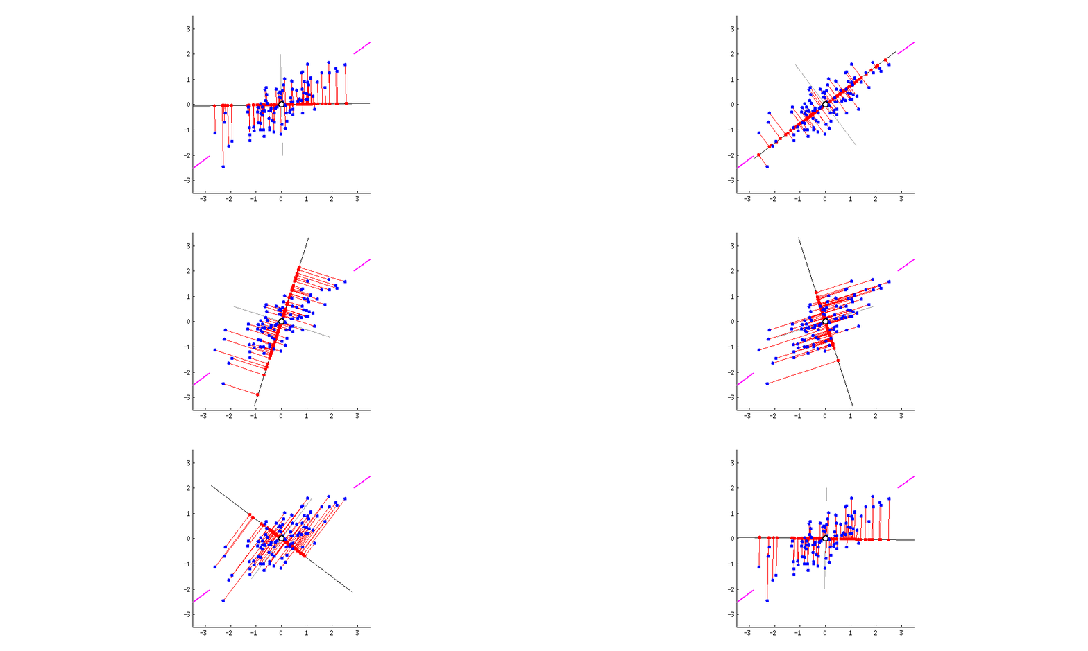
PCA can be interpreted visually. Imagine a dataset with two attributes plotted in a 2D space. The first principal component would be a line that maximizes the spread (or, mathematically speaking, variance) of the data points projected on that line (see image below). The second component would be a similar line, perpendicular to the first.

One disadvantage worth noting is that final principal components are very difficult (or impossible) for humans to interpret. Depending on the circumstances, this may cause PCA to be inapplicable.
Putting PCA into Practise
An example of the effective use of PCA was our recent project on the automatic classification of job applicants. The initial attribute space proved to be rather big and the first results, while acceptable, could still be improved. By using PCA, we managed to relevantly reduce the number of dimensions and consequently increase classification performance. Furthermore, the time needed to learn the model was reduced. Both of these improvements are very welcomed, especially when the training phase takes days or even months, like in the case of deep neural networks.
Find the Best Approach to Dimensionality Reduction for You
PCA is an effective, fast, and readily available feature reduction technique commonly used in machine learning. The most common implementation is available in the Scikit-Learn Python library. As a Data Scientist, I highly encourage everyone to test it in their projects. Of course, there are many more sophisticated approaches to dimensionality reduction – among the most flashy ones are t-SNE and UMAP. You can experiment with them live using the fantastic Tensorflow Projector at https://projector.tensorflow.org/.
Keywords: machine learning, data, dimensionality reduction, feature engineering, feature selection, principal component analysis, curse of dimensionality, model performance
Read more about PCA: https://builtin.com/data-science/step-step-explanation-principal-component-analysis
Learn about t-SNE: https://distill.pub/2016/misread-tsne
Implementations:
PCA: https://scikit-learn.org/stable/modules/generated/sklearn.decomposition.PCA.html
UMAP: https://umap-learn.readthedocs.io/en/latest/index.html
t-SNE: https://scikit-learn.org/stable/modules/generated/sklearn.manifold.TSNE.html


